Contents
Electrode voltage profile for piezoelectric sensor
Introduction
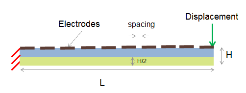
The Reference mentioned below solved the piezoelectric problem in actuation mode. This problem solves for the same problem shown in the Reference but now in sensor mode. 10 equally spaced electrodes are placed on top as shown in the picture below. A vertical tip displacement is specified and the voltages on the electrodes are measured. This problem
- Solves the piezoelectric problem in actuation mode and measures voltages in response to a vertical displacement
- Specifies linear constitutive equations for PVDF using Symbolic Math Toolbox (R2012b or greater)
- Shows a convenient way to specify constrained (tied) BCs
- Shows a way to specify a BC value at a node
Requirements: PDE Toolbox, Helper classes for PDE Toolbox, Symbolic Math Toolbox (R2012b and greater)
References : http://www.mathworks.com/help/pde/examples/deflection-of-a-piezoelectric-actuator.html
%
function piezoSensor
import pdetbplus.*; % use helper classes
Geometry
L = 50e-3;
H = 1e-3;
% specify boundaries
p{1} = pointObject(0,0);
p{2} = pointObject(0,H/2);
a{1} = lineObject('wall1',p{1},p{2});
% specify electrode boundaries
numElectrodes  = 10;
spacing = H/20;
electrodeLength = (L-(numElectrodes-1)*spacing)/numElectrodes;
for k=1:numElectrodes-1
    p{end+1} = pointObject(k*electrodeLength,H/2);
    a{end+1} = lineObject(strcat('electrode',num2str(k)),p{end-1},p{end});
    p{end+1} = p{end} + [spacing,0];
    a{end+1} = lineObject(strcat('gapElectrode',num2str(k)),p{end-1},p{end});
end
p{end+1} = pointObject(L,H/2);
% boundary for final electrode
a{end+1} = lineObject('electrode10',p{end-1},p{end});
p{end+1} = pointObject(L,0);
a{end+1} = lineObject('free1',p{end-1},p{end});
for k=1:length(a)
    a{k}.leftRegion = 'nonMeshedSpace';
    a{k}.rightRegion = 'beamMaterial1'; % there are two regions to the beam
end
a{end+1} = lineObject('separator',p{end},p{1});
a{end}.leftRegion = 'beamMaterial2';
a{end}.rightRegion = 'beamMaterial1';
topPartLength = length(a);
% boundaries for lower part
p{end+1} = pointObject(L,-H/2);
a{end+1} = lineObject('free2',p{end-1},p{end});
p{end+1} = pointObject(0,-H/2);
a{end+1} = lineObject('bottom',p{end-1},p{end});
a{end+1} = lineObject('wall2',p{end},p{1});
for k=topPartLength+1:length(a)
    a{k}.leftRegion = 'nonMeshedSpace';
    a{k}.rightRegion = 'beamMaterial2';
end
% create geometries
beamTop = geometryObject('beamTop',a(1:topPartLength));
beamBottom = geometryObject('beamBottom',a(topPartLength+1:end));
beam = beamTop + beamBottom;
beam.exteriorRegion = 'nonMeshedSpace';
beam = beam.initMesh('showMesh',true,'Hmax',H/5); axis('equal');
warning: Approximately 2500 triangles will be generated.
Boundary conditions
N = 3; % output dimension
% instantiate boundaryConditionObject for convenient definition of BCs
bc = boundaryConditionObject(beam, N);
    function [hval,rval,qval,gval] = bcondWall(x,y,u,t)
        % Dirichlet condition on the boundary
        rval = zeros(N,1);
        hval = speye(N); % u,v are zero on wall
        hval(3,3) = 0;
        qval = [];
        gval = [];
    end
    function [hval,rval,qval,gval] = bcondBottom(x,y,u,t)
        % Dirichlet condition on the boundary
        rval = zeros(N,1);
        hval = sparse(N,N);
        hval(3,3) = 1; % potential is 0 on bottom boundary
        qval = [];
        gval = [];
    end
    function [hval,rval,qval,gval] = bcondFree(x,y,u,t)
        % Dirichlet condition on the boundary
        rval = zeros(N,1);
        hval = sparse(N,N);
        qval = [];
        gval = [];
    end
bc.add('name','free1','xyutFunction',@bcondFree);
bc.add('name','free2','xyutFunction',@bcondFree);
bc.add('name','wall1','xyutFunction',@bcondWall);
bc.add('name','wall2','xyutFunction',@bcondWall);
bc.add('name','bottom','xyutFunction',@bcondBottom);
[Qmat,Gmat,Hmat,Rmat] = bc.getMatrices(); % global BC matrices so far
% additional BC matrices for setting voltages on electrode to be the same
Hadd = [];
Radd = [];
for k=1:numElectrodes
    electrodeName = strcat('electrode',num2str(k));
    % tie voltage i.e. 3rd dimension to be same on boundary electrodeName
    [HaddInc,RaddInc] = bc.getGlobalHR('name',electrodeName,'type','tie','dimension',3);
    Radd = [Radd;RaddInc];
    Hadd = [Hadd;HaddInc];
end
% combine global BC matrices
Hmat = [Hmat;Hadd];
Rmat = [Rmat;Radd];
% final BC for point load
freeBoundaryNodes = beam.getBoundaryNodes('name','free1'); % get all boundary nodes on free1
[~,ix] = max(beam.mesh.p(2,freeBoundaryNodes)); % node with maximum y coordinate i.e. tip node
pointDisplacementNode = freeBoundaryNodes(ix); % find node of interest
% set a vertical displacement of -10e-3 at tip
[HaddPointDisplacement,RaddPointDisplacement] = bc.getGlobalHR('type','point','nodes',pointDisplacementNode,'value',-10e-3,'dimension',2);
HmatComplete = [Hmat;HaddPointDisplacement];
RmatComplete = [Rmat;RaddPointDisplacement];
Coefficients
numNodes = size(beam.mesh.p,2);
% create functions out of frequency domain piezoelectric equations
% Define piezoelectric equations (strain-charge formulation) using Symbolic Math Toolbox; To avoid errors, make
% this function standalone instead of a nested function
function [equations,variables] = piezoEquationsFreq(varargin)
displayEquations = true;
E = 0;nu = 0;G = 0;d31 = 0;d33 = 0;epsr = 0;rho = 0;s = 0;eps0 = 8.854187817620e-12;
for k=1:2:length(varargin)
  a = varargin(k);
  b = varargin(k+1);
  if strcmp(a,'E')
      E = b{1};
  elseif strcmp(a,'nu')
      nu = b{1};
  elseif strcmp(a,'G')
      G = b{1};
  elseif strcmp(a,'d31')
      d31 = b{1};
  elseif strcmp(a,'d33')
      d33 = b{1};
  elseif strcmp(a,'epsr')
      epsr = b{1};
  elseif strcmp(a,'rho')
      rho = b{1};
  elseif strcmp(a,'s')
      s = b{1};
  elseif strcmp(a,'displayEquations')
      displayEquations = b{1};
  end
end
if G == 0
   G = E/(2*(1+nu));
end
%% PDE input, define eq and input;
% *Reserved keywords: x,y,time,ddx,ddy,d[variable]dx,d[variable]dy*
% *specify the Div operator as [ddx ddy]
syms ddx ddy real;
% user input begins
syms u v dudx dudy dvdx dvdy real;
%% material constants
C11 = E/(1-nu^2);
C12 = C11*nu; C21=C12;
C22 = C11;
C66 = G;
%% Linear strain tensor
epsilon11 = dudx;
epsilon22 = dvdy;
epsilon12 = (dudy+dvdx)/2;
%% stress equations
Sx = C11*epsilon11 + C12*epsilon22;
Sy = C21*epsilon11 + C22*epsilon22;
Txy = C66*2*epsilon12; % watch out for factor of 2 for engineering strain
strainStress = [Sx;Sy;Txy];
% The piezoelectric strain coefficients for PVDF
% The notation of the d matrix is different from those in standard references
% the "3" in dn3 below is not the z direction but is the y direction.
d = [0 d31; 0 d33; 0 0];
syms E1 E2 phi dphidx dphidy xi D real;
E1 = -dphidx;
E2 = -dphidy;
C = [C11 C12 0;C12 C22 0;0 0 C66];
e = C*d;
pzeStress = -e*[E1;E2];
stressSigma = strainStress + pzeStress; % linearized stress
stress = [stressSigma(1) stressSigma(3);stressSigma(3) stressSigma(2)];
permitt = eps0*epsr*eye(2); % constant stress permittivity matrix
permitt = permitt - d.'*(C\d); % constant strain permittivity matrix
D = (e'*[epsilon11;epsilon22;2*epsilon12] + permitt*[E1;E2]); % electric displacement equation
equations = -[ddx ddy]*[stress D] + s^2*rho*[u v 0]; % the PDE
if displayEquations
  display Problem_Equations;
  equations'
end
variables = [u v phi];
end
piezoEquations1 = @() piezoEquationsFreq('E',2e9,'nu',0.29,'G',0.775e9,'d31',2.2e-11','d33',-3e-11,'epsr',12,'s',0);
% flip sign of d31 and d33
piezoEquations2 = @() piezoEquationsFreq('E',2e9,'nu',0.29,'G',0.775e9,'d31',-2.2e-11','d33',3e-11,'epsr',12,'s',0);
coeff = coeffsObject(beam, N);
coeff.add('region','beamMaterial1','symbolicEquationFunction',piezoEquations1); % requires Symbolic Math Toolbox
coeff.add('region','beamMaterial2','symbolicEquationFunction',piezoEquations2); % requires Symbolic Math Toolbox
[Kmat,Mmat,Fmat] = coeff.getMatrices('u',zeros(N*numNodes,1));
Problem_Equations

ans =

                         - ddy*(775000000*dudy + 775000000*dvdx) - ddx*((266*dphidy)/9159 + (4579434436073807*dudx)/2097152 + (332008996615351*dvdy)/524288)
                       - ddx*(775000000*dudy + 775000000*dvdx) - ddy*((332008996615351*dudx)/524288 - (2362*dphidy)/45795 + (4579434436073807*dvdy)/2097152)
 (4110357605544239*ddx*dphidx)/38685626227668133590597632 + ddy*((4110357605544239*dphidy)/38685626227668133590597632 - (266*dudx)/9159 + (2362*dvdy)/45795)

Cmatrix

  +-                                                                                                                                                               -+
  |  4579434436073807/2097152,     0,         0,      5800000000000/9159,                       0,                                       266/9159                   |
  |                                                                                                                                                                 |
  |              0,            775000000, 775000000,          0,                                0,                                           0                      |
  |                                                                                                                                                                 |
  |   332008996615351/524288,      0,         0,     20000000000000/9159,                       0,                                      -2362/45795                 |
  |                                                                                                                                                                 |
  |              0,                0,         0,              0,          -4110357605544239/38685626227668133590597632,                      0                      |
  |                                                                                                                                                                 |
  |          266/9159,             0,         0,         -2362/45795,                           0,                      -957406751230359/9010865545125641773383680  |
  +-                                                                                                                                                               -+
Fvector

  +-       -+
  | 0, 0, 0 |
  +-       -+
Problem_Equations

ans =

                         - ddy*(775000000*dudy + 775000000*dvdx) - ddx*((4579434436073807*dudx)/2097152 - (266*dphidy)/9159 + (332008996615351*dvdy)/524288)
                       - ddx*(775000000*dudy + 775000000*dvdx) - ddy*((2362*dphidy)/45795 + (332008996615351*dudx)/524288 + (4579434436073807*dvdy)/2097152)
 (4110357605544239*ddx*dphidx)/38685626227668133590597632 + ddy*((4110357605544239*dphidy)/38685626227668133590597632 + (266*dudx)/9159 - (2362*dvdy)/45795)

Cmatrix

  +-                                                                                                                                                               -+
  |  4579434436073807/2097152,     0,         0,      5800000000000/9159,                       0,                                       -266/9159                  |
  |                                                                                                                                                                 |
  |              0,            775000000, 775000000,          0,                                0,                                           0                      |
  |                                                                                                                                                                 |
  |   332008996615351/524288,      0,         0,     20000000000000/9159,                       0,                                      2362/45795                  |
  |                                                                                                                                                                 |
  |              0,                0,         0,              0,          -4110357605544239/38685626227668133590597632,                      0                      |
  |                                                                                                                                                                 |
  |          -266/9159,            0,         0,          2362/45795,                           0,                      -957406751230359/9010865545125641773383680  |
  +-                                                                                                                                                               -+
Fvector

  +-       -+
  | 0, 0, 0 |
  +-       -+
Solve
% matrix form of assempde() is needed because of the global BC on the
% electrodes
u = assempde(Kmat,Mmat,Fmat,Qmat,Gmat,HmatComplete,RmatComplete);
Post-process
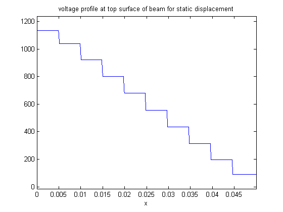
% plot potential on top surface
uu = reshape(u(1:3*numNodes),numNodes,[]);
phixy = beam.createXYFunctionFromNodalSolution(uu(:,3)); % x,y voltage function
phiTop = @(x) abs(phixy(x,H/2-eps)); % top surface voltage function
figure(1);ezplot(phiTop,[0,L-eps]); title 'voltage profile at top surface of beam for static displacement';% plot voltage on top surface
Documentation of classes
See help for geometryObject lineObject pointObject coeffsObject boundaryConditionObject
More info and other examples
end