motor

Magnetostatic analysis of a Switched Reluctance Motor
Define parameter defaults and read in variables
Define geometry : rotor and stator
Plot geometry
Formulation dimension
Add BC
Mesh
Coefficients
Solve
Post process
Calculate torque using Maxwell stress method
Calculate co-energy
Documentation of classes
More info and other examples

Magnetostatic analysis of a Switched Reluctance Motor

Introduction

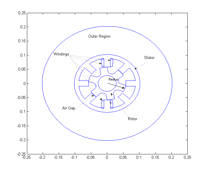
Basic geometry from Switched-Reluctance Motor Torque Characteristics: Finite-Element Analysis and Test Results G. E. Dawson, A. R. Eastham, J. Mizia, IEEE TRANSACTIONS ON INDUSTRY APPLICATIONS, VOL. IA-23, NO. 3, MAY/JUNE 1987

What does it do? : The demo uses the PDE toolbox to solve the magnetostatic PDE : $-\nabla^2 (\mu A) = J$ (A: magnetic potential, mu : magnetic permeability and J : current density) on the geometry of a switched reluctance motor for a specified design point: airGap, relative magnetic permeability (muMetal), #winding turns, stackDepth and rotorRadius. It returns the static torque and coenergy for the design point and plots the B field. Only linear permeable material is considered for the metal part with a constant muMetal value. However, you can modify the script to specify a nonlinear permeability.

There are two modes of running:

  1. Run motor() with the default design point or with an input design point such as motor('rotateAngle',pi/4,...).
  2. Run motorGUI() to perform parametric analysis and plot the torque and co-energy curves. motorGUI() calls motor() per design point.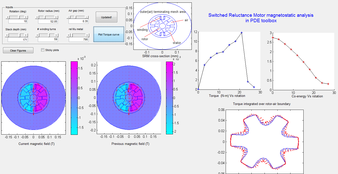

Further Instructions for motorGUI

run "motorGUI.m". This launches motorGUI.fig - a GUIDE developed frontend around the function motor().
click on "Click to Update!" for performing individual point simulation based on the parametric inputs - Rotation angle, rotor radius etc
click on "Plot Torque curve" to product Torque and Coenergy curves

See exampleGeometries.m and exampleFormulation.m on how to use the GeometryObject and the other classes used in this example

Requirements: PDE Toolbox, the package pdetbplus

function [rotorPart,statorPart,torque,coenergy] = motor(varargin)

import pdetbplus.*; % import package for accessing the geometryObject, boundary (arcObject etc), boundaryConditionObject and coeffsObject classes

Define parameter defaults and read in variables

rotateAngle = pi/9; % radians
rotorRadius = 58.05; % mm
airGap = 0.35; % mm
stackDepth = 171; % in mm
murMetal = 795; % low magnetic permeability
numberOfTurns = 59; % number of turns in the winding
rotorPart = []; % geometry part corresponding to the rotor
statorPart = []; % geometry part corresponding to the stator
returnAfterPlotGeometry = false; % set to true if motor() should return after just plotting geometry
showPostProcessIntegrationBoundary = false;
figureHandle = [];
plotFigureAxes = [];
postProcessIntegrationBoundaryAxes = [];
for k=1:2:length(varargin)
    a = varargin(k);
    b = varargin(k+1);
    if strcmp(a,'rotateAngle')
        rotateAngle = b{1};
    elseif strcmp(a,'rotorRadius')
        rotorRadius = b{1};
    elseif strcmp(a,'rotorPart')
        rotorPart = b{1};
    elseif strcmp(a,'statorPart')
        statorPart = b{1};
    elseif strcmp(a,'airGap')
        airGap = b{1};
    elseif strcmp(a,'murMetal')
        murMetal = b{1};
    elseif strcmp(a,'numberOfTurns')
        numberOfTurns = b{1};
    elseif strcmp(a,'stackDepth')
        stackDepth = b{1};
    elseif strcmp(a,'returnAfterPlotGeometry')
        returnAfterPlotGeometry = b{1};
    elseif strcmp(a,'showPostProcessIntegrationBoundary')
        showPostProcessIntegrationBoundary = b{1};
    elseif strcmp(a,'returnAfterPlotGeometry')
        figureHandle = b{1};
    elseif strcmp(a,'plotFigureAxes')
        plotFigureAxes = b{1};
    elseif strcmp(a,'postProcessIntegrationBoundaryAxes')
        showPostProcessIntegrationBoundary = true;
        postProcessIntegrationBoundaryAxes = b{1};
    end
end
% Prepare figures, axes
if isempty(figureHandle)
    figureHandle = get(0,'CurrentFigure');;
end
if isempty(plotFigureAxes)
    plotFigureAxes = get(figureHandle,'CurrentAxes');
else
    figure(figureHandle);
    axes(plotFigureAxes);
end
if showPostProcessIntegrationBoundary
    if isempty(postProcessIntegrationBoundaryAxes)
        postProcessIntegrationBoundaryFigure = figure(2);
        postProcessIntegrationBoundaryAxes = gca;
    else
        postProcessIntegrationBoundaryFigure = figureHandle;
    end
end

Define geometry : rotor and stator

statorRadius = rotorRadius + airGap; % mm
if nargin < 2 || isempty(rotorPart) || isempty(statorPart)
    rotorPart = rotor(rotorRadius, 'air'); % look into rotor() to see what region names are defined
    statorPart = stator(statorRadius); % look into stator() to see what region names are defined
end
center = pointObject(0.0,0.0);
rotorPartRotated = rotorPart.rotate(center,rotateAngle);
assembly = statorPart + rotorPartRotated;
assembly.exteriorRegion = statorPart.exteriorRegion; % happens to be 'outer'
assembly = assembly.scale(1e-3); % convert mm to m
stackDepth = stackDepth*1e-3; % convert mm to m

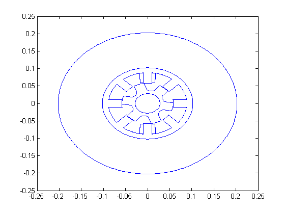
Plot geometry

assembly.plot();
if returnAfterPlotGeometry
    torque = [];
    coenergy = [];
    return;
end

Formulation dimension

outputDimension = 1;

Add BC

    function [hval,rval,qval,gval] = bcond(x,y,u,t)
        % Dirichlet condition on the boundary
        rval(1) = 0;
        hval(1) = 1;
        qval = [];
        gval = [];
    end
% instantiate boundaryConditionObject for convenient definition of BCs
bc = boundaryConditionObject(assembly, outputDimension);
outsideBCRegionName = 'nonMeshedSpace';
insideBCRegionName = 'outer'; % this region was defined in stator()
% BC specified between nonMeshedSpace and outer (the outermost annulus)
bc.add('outerRegion',outsideBCRegionName,'innerRegion',insideBCRegionName,'xyutFunction',@bcond);

Mesh

assembly = assembly.initMesh('showMesh',false);
showRegion = false;
if showRegion
    % plot individual regions; Note: because of limitation in plot() should
    % be called after meshing
    for k=1:length(assembly.regions)
        figure(k);
        assembly.plotRegion(assembly.regions{k});
    end
end

Coefficients

current Density, J = 10 Amps X number of turns / windingArea

windingArea = assembly.getRegionArea('winding1'); % winding1 area equal to other winding areas.
currentDensity = -10*numberOfTurns/windingArea;
fcoeffMOne = @(x,y,u,ux,uy,time) currentDensity;
fcoeffOne = @(x,y,u,ux,uy,time)  -currentDensity;
% instantiate coeffsObject for convenient definition of coefficients
coeff = coeffsObject(assembly, outputDimension);
% use linear permeable materials
murel = 4*pi*1e-7; % magnetic permeability of free space
cfreespace = 1/murel;
cmetal = 1/(murMetal*murel);
    function c = ccoeffMetal(x,y,u,ux,uy,time)
        c = [cmetal 0;0 cmetal];
    end
% specify ccoeffMetal() for regions where it is valid; regions referred below were defined in rotor() and stator()
coeff.add('region','rotor','cijFunction',@ccoeffMetal);
coeff.add('region','stator','cijFunction',@ccoeffMetal);
coeff.add('region','core','cijFunction',@ccoeffMetal);
    function c = ccoeffFreeSpace(x,y,u,ux,uy,time)
        c = [cfreespace 0;0 cfreespace];
    end
% free space coefficient for the other regions
coeff.add('region','winding1','fiFunction',fcoeffMOne,'cijFunction',@ccoeffFreeSpace);
coeff.add('region','winding2','fiFunction',fcoeffOne,'cijFunction',@ccoeffFreeSpace);
coeff.add('region','winding3','fiFunction',fcoeffOne,'cijFunction',@ccoeffFreeSpace);
coeff.add('region','winding4','fiFunction',fcoeffMOne,'cijFunction',@ccoeffFreeSpace);
coeff.add('region','air','cijFunction',@ccoeffFreeSpace);
coeff.add('region','outer','cijFunction',@ccoeffFreeSpace);

Solve

a = 0; % magnetostatic problem
numAdaptivePasses = 5;
[A,p,e,t] = adaptmesh(assembly.geometryFunction, bc.bcFunction,coeff.cFunction,a,coeff.fFunction,'Ngen',numAdaptivePasses);
% reset mesh object since adaptmesh changes mesh size
assembly.mesh = meshObject('p',p,'e',e,'t',t);

Number of triangles: 8910
Number of triangles: 8954
Number of triangles: 9134
Number of triangles: 9174
Number of triangles: 9458
Number of triangles: 9526

Maximum number of refinement passes obtained.

Post process

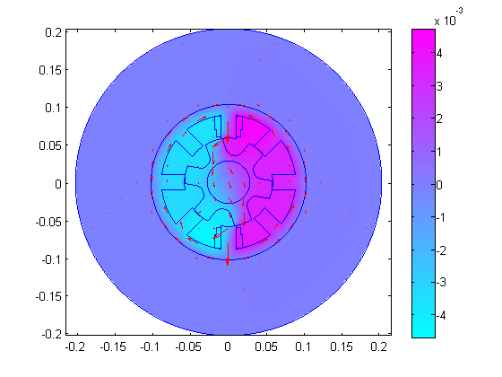
calculate $B = \nabla \times A$

[dAdx,dAdy] = pdegrad(assembly.mesh.p,assembly.mesh.t,A);
Bx = dAdy;
By = -dAdx;
hold on;
pdeplot(assembly.mesh.p, assembly.mesh.e, assembly.mesh.t, 'xydata', A, 'contour','off','colorbar','on','mesh','off','flowdata',[Bx;By]); axis equal;

Calculate torque using Maxwell stress method

Magnetic field intensity $H = \mu B$ ; but we calculate H from pdecgrad() for convenience

[cdAdx,cdAdy] = pdecgrad(assembly.mesh.p,assembly.mesh.t,@coeff.cFunction,A);
Hx = cdAdy;
Hy = -cdAdx;
    function dT = differentialTorque(xmid,ymid,nxmid,nymid,inputs)
        bx = inputs{1};
        by = inputs{2};
        hx = inputs{3};
        hy = inputs{4};
        % dT = (position X H)(n.B) + (position X B)(n.H) - (position X n)(H.B)
        dT3 = 0.5*((xmid*hy-ymid*hx)*(nxmid*bx+nymid*by) + (xmid*by-ymid*bx)*(nxmid*hx+nymid*hy) - (xmid*nymid-ymid*nxmid)*(bx*hx+by*hy));
        dT = [0 0 dT3]';
    end
if nargout > 1
    if showPostProcessIntegrationBoundary
        figure(postProcessIntegrationBoundaryFigure);
        axes(postProcessIntegrationBoundaryAxes);
    end
    % integrate torque differential dT over air-rotor boundary but still on
    % the air side
    torque = assembly.integrateOutsideBoundary('innerRegion','rotor','outerRegion','air','integrand',@differentialTorque,'showBoundary',showPostProcessIntegrationBoundary,Bx,By,Hx,Hy)*stackDepth;
    axes(plotFigureAxes);
else
    torque = [];
end

Calculate co-energy

    function dC = differentialCoenergyPart1a(xmid,ymid,inputs)
        % avector = [0 0 inputs{1}];
        % J = [0 0 currentDensity];
        % dC = dot(avector,J);
        dC = inputs{1}*currentDensity;
    end
    function dC = differentialCoenergyPart1b(xmid,ymid,inputs)
        % avector = [0 0 inputs{1}];
        % J = [0 0 -currentDensity];
        % dC = dot(avector,J);
        dC = inputs{1}*(-currentDensity);
    end
    function dC = differentialCoenergyPart2(xmid,ymid,inputs)
        bx = inputs{1};
        by = inputs{2};
        hx = inputs{3};
        hy = inputs{4};
        % dC = 0.5*dot(B,H);
        dC = 0.5*(bx*hx+by*hy);
    end
% interpolate A from mesh vertices to centroids of mesh elements
Atriangles = pdeintrp(assembly.mesh.p,assembly.mesh.t,A);
% integrate differentialCoenergyPart1a/b() over the windings (where
% the current density contribution exists)
coenergy1 = assembly.integrateOverRegion('integrand',@differentialCoenergyPart1a,'region','winding1','integrandInput',{Atriangles});
coenergy1 = assembly.integrateOverRegion('integrand',@differentialCoenergyPart1b,'region','winding2','integrandInput',{Atriangles}) + coenergy1;
coenergy1 = assembly.integrateOverRegion('integrand',@differentialCoenergyPart1a,'region','winding4','integrandInput',{Atriangles}) + coenergy1;
coenergy1 = assembly.integrateOverRegion('integrand',@differentialCoenergyPart1b,'region','winding3','integrandInput',{Atriangles}) + coenergy1;
coenergy1 = coenergy1*stackDepth;
% integrate differentialCoenergyPart2() over all regions
coenergy2 = 0;
for k=1:length(assembly.regions)
    coenergy2 = assembly.integrateOverRegion('integrand',@differentialCoenergyPart2,'region',assembly.regions{k},'integrandInput',{Bx,By,Hx,Hy}) + coenergy2;
end
coenergy2 = coenergy2 * stackDepth;
coenergy = coenergy1 - coenergy2;

Documentation of classes

See help for geometryObject lineObject arcObject pointObject coeffsObject boundaryConditionObject meshObject

More info and other examples

See other examples

end

ans = 

  pdetbplus.geometryObject
  Package: pdetbplus

  Properties:
                name: 'rotor'
      exteriorRegion: 'air'
                mesh: [1x1 pdetbplus.meshObject]
            boundary: {1x36 cell}
             regions: {'air'  'core'  'rotor'}
    geometryFunction: @(varargin)self.geometryFunction_impl(varargin{:})
          regionToId: [3x1 containers.Map]

Contents