Contents
Solve Laplace's equation with periodic boundary conditions on octagon shaped geometry
Introduction
Laplace's equation  is solved on an octagon. Sides 8 and 4 are constrained with periodic BCs. Further Side 8 has a varying BC.
function examplePeriodicBC
import pdetbplus.*; % import package for accessing the geometryObject, boundaryConditionObject and coeffsObject classes
Geometry
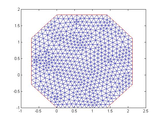
% Points of the octagon
p{1} = pointObject(0,0);
p{2} = pointObject(1,1);
p{3} = pointObject(2,1);
p{4} = pointObject(3,0);
p{5} = pointObject(3,-1);
p{6} = pointObject(2,-2);
p{7} = pointObject(1,-2);
p{8} = pointObject(0,-1);
% Create polygon with inside region called 'tissue' and outside region called 'cavity'. 'cavity' is
% not meshed.
g = geometryObject.createPolygon('name','Octo','points',p,'leftRegion','cavity','rightRegion','tissue',...
    'leftRegionIsExterior',true);
g.exteriorRegion = 'cavity';
% Rotate geomety around (0,-1) anti-clockwise by 45 degrees
g = g.rotate(pointObject(0,-1),pi/4);
% Mesh
g = g.initMesh('showMesh',true,'numRefineMeshSteps',1);
% Set dimension of the problem to 1
N = 1;
Boundary Conditions
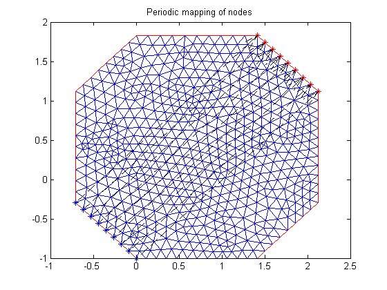
% Instantiate boundary condition object
bc = boundaryConditionObject(g,N);
% Add varying BC to boundary{8}
    function [hval,rval,qval,gval] = varyWithY(x,y,u,t)
        qval = [];
        gval = [];
        hval = 1;
        rval = y;
    end
bc.add('name',g.boundary{8}.name,'xyutFunction',@varyWithY);
% Get global matrices corresponding to BC's defined so far
[Q,G,H,R] = bc.getMatrices();
% Get contribution to global H,R matrices for periodicity condition between a pair of opposite boundaries
hold on; % for plotting periodic mapping of nodes
[Hadd,Radd] = bc.getGlobalHR('name',g.boundary{8}.name,'dimension',1,'type','periodic',...
    'periodicX','x+3*cos(pi/4)','periodicY','y+3*sin(pi/4)','showNodes',true);
title 'Periodic mapping of nodes';
snapnow;
% Combine the additional H,R matrices
H = [H;Hadd];
R = [R;Radd];
Coefficient
coeffs = coeffsObject(g,N);
% Define Laplace's equation
coeffs.add('region','tissue','cConstantValue',1,'fConstantValue',0);
% Extract matrices
[K,M,F] = coeffs.getMatrices();
Solve
% Solve using matrix form of assempde
u = assempde(K,M,F,Q,G,H,R);
Plot
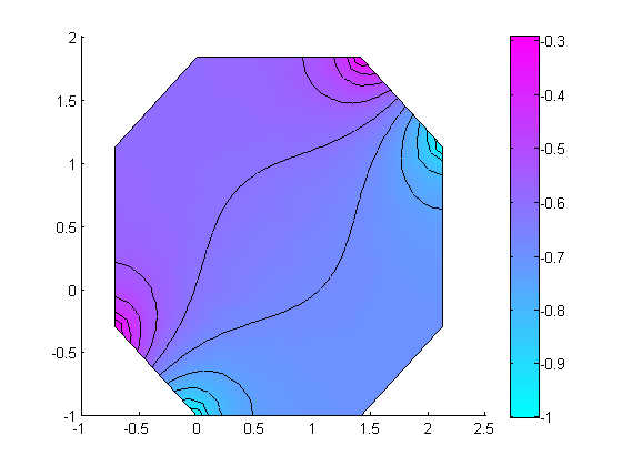
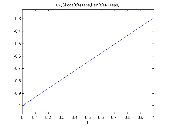
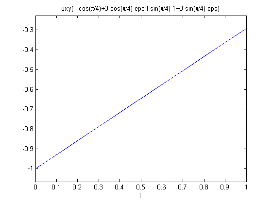
% Plot contour of solution
clf;
pdeplot(g.mesh.p,g.mesh.e,g.mesh.t,'xydata',u,'contour','on','mesh','off');
snapnow;
% Verify plots of solution on the periodic boundary pair are the same
uxy = g.createXYFunctionFromNodalSolution(u);
% Create plot on left boundary; eps is added/subtracted to make sure plot is inside region
u_left = @(l) uxy(-l*cos(pi/4)+eps, l*sin(pi/4)-1+eps);
ezplot(u_left,[0,1]);
snapnow;
% Create plot on periodic boundary; eps is added/subtracted to make sure plot is inside region
u_periodic = @(l) uxy(-l*cos(pi/4)+3*cos(pi/4)-eps, l*sin(pi/4)-1+3*sin(pi/4)-eps);
ezplot(u_periodic,[0,1]);
snapnow;
Documentation of classes
See help for geometryObject pointObject coeffsObject boundaryConditionObject meshObject
More info and other examples
end