Contents
- Solve Laplace's equation on a 4-sided polygon
- Define geometry using geometryObject class
- Define boundary conditions using boundaryConditionObject class
- Define coefficients using coeffsObject class
- Solve
- Post-process : integration on boundary and area
- Post-process: Create and use
 function from solution
- Documentation of classes
- More info and other examples
Solve Laplace's equation on a 4-sided polygon
Introduction
Laplace's equation  is solved on a 4-sided polygon domain. Sides 1 and 3 have Dirichlet BC,
  , sides 2 and 4 have Neumann BC,
function exampleFormulation
import pdetbplus.*; % import package for accessing the geometryObject, boundaryConditionObject and coeffsObject classes
Define geometry using geometryObject class
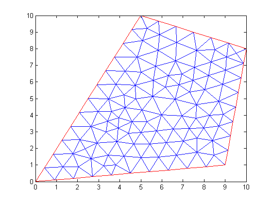
Define geometry and mesh it.
% Start by defining points of the polygon
pts{1} = pointObject(0.0,0.0);
pts{2} = pointObject(5,10);
pts{3} = pointObject(10,8);
pts{4} = pointObject(9,1);
% Specify the inside and outside regions
leftRegion = 'air';
rightRegion = 'fooMaterial';
% Close polygon
leaveOpen = false;
% Left region is exterior
leftRegionIsExterior = true;
g = geometryObject.createPolygon('name','fooPolygon','points',pts,'leftRegion',leftRegion,'rightRegion',rightRegion,...
    'leftRegionIsExterior',leftRegionIsExterior,'leaveOpen',leaveOpen);
% Although exterior region has been set, good practice to set it explicitly
g.exteriorRegion = 'air';
figure(1);
g = g.initMesh('showMesh',true); % note this is an initial mesh that could be changed by adaptmesh()
% Set dimension of the problem to 1
N = 1;
Define boundary conditions using boundaryConditionObject class
% Instantiate boundary condition object
bc = boundaryConditionObject(g,N);
% Use built in Dirichlet option
bc.add('name',g.boundary{1}.name,'dirichlet',5);
bc.add('name',g.boundary{3}.name,'dirichlet',0);
% Specifying Neumann BC can be skipped since it is a natural BC.
% However it is set below in 2 different ways for illustration.
bc.add('name',g.boundary{2}.name,'neumann',0);
% BC can also be specified in terms of a function for more flexibility
  function [hval,rval,qval,gval] = bcondNeumann(x,y,u,t)
        rval = [];
        hval = [];
        qval = sparse(N,N);
        gval = zeros(N,1);
    end
bc.add('name',g.boundary{4}.name,'xyutFunction',@bcondNeumann);
Define coefficients using coeffsObject class
coeffs = coeffsObject(g,N);
% Specify coefficients using functions.
% Since we are solving a Laplace problem "a" coefficient is zero
% Define "c" coefficient
    function cij = cCoeff(x,y,u,ux,uy,time) % receive x,y,y,ux,uy at centroids
        cij = [1 0; 0 1];
    end
    function fi = fCoeff(x,y,u,ux,uy,time) % receive x,y,y,ux,uy at centroids
        fi = zeros(N,1);
    end
    function aij = aCoeff(x,y,u,ux,uy,time) % receive x,y,y,ux,uy at centroids
        aij = zeros(N,N);
    end
% Add coefficient functions
coeffs.add('region','fooMaterial','fiFunction',@fCoeff,'cijFunction',@cCoeff,'aijFunction',@aCoeff);
Solve
% Supply initial guess even though problem is linear
u0 = zeros(size(g.mesh.p,2),1);
[u,p,e,t] = adaptmesh(g.geometryFunction,bc.bcFunction,coeffs.cFunction,coeffs.aFunction,coeffs.fFunction,'Init',u0,'Ngen',1);
% Reset mesh in g, since adaptive mesh changed mesh size
g.mesh = meshObject('p',p,'e',e,'t',t);
Number of triangles: 198
Number of triangles: 238

Maximum number of refinement passes obtained.
Post-process : integration on boundary and area
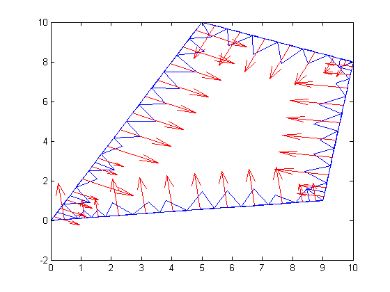
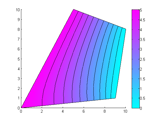
% Integrate ||c grad u.n||^2 along boundary of region
% Define boundary integrand.
    function val = integrandNeumann(xmid,ymid,nxmid,nymid,inputs)
        ux = inputs{1};
        uy = inputs{2};
        val = (ux*nxmid + uy*nymid)^2;
    end
% Get c grad u
[cdudx,cdudy] = pdecgrad(g.mesh.p,g.mesh.t,coeffs.cFunction,u);
% Notice how inner region is specified as 'air' below because integration
% is done 'outside' a boundary. Since there are no triangles in air and there are triangles in the interior region, we
% flip the meaning of the inner and outer regions
figure(2);
% Integrate
val1 = g.integrateOutsideBoundary('innerRegion','air','outerRegion','fooMaterial','integrand',@integrandNeumann,...
    'showBoundary',true,'showBoundaryClear',false,'integrandInput',{cdudx,cdudy});
g.plot(); %overlay geometry
fprintf('||grad u.n||^2 along air-material boundary = %e \n',val1);

% Integrate u*sqrt(x^2+y^2) on region using geometryObject class
% Define region integrand.
    function val = integrandSegs(xmid,ymid,inputs)
        umid = inputs{1};
        val = umid*sqrt(xmid^2+ymid^2); % some function
    end
% Interpolate u from mesh vertices to centroids of mesh elements
utriangles = pdeintrp(g.mesh.p,g.mesh.t,u);
% Integrate
val2 = g.integrateOverRegion('integrand',@integrandSegs,'region','fooMaterial','integrandInput',{utriangles});
fprintf('integral of distance weighted solution = integral(sqrt(x^2+y^2)*u) over interior region = %e\n',val2);
% Plot
figure(3);
pdeplot(g.mesh.p, g.mesh.e, g.mesh.t, 'xydata', u, 'contour', 'on');
||grad u.n||^2 along air-material boundary = 9.866139e+00
integral of distance weighted solution = integral(sqrt(x^2+y^2)*u) over interior region = 1.170931e+03
Post-process: Create and use function from solution
Integrate  on a horizontal line (2,4) and (pt2x,4) between first and third boundaries. Height of the line is 4. Create solution as a function of (x,y)
uxy = g.createXYFunctionFromNodalSolution(u);
% Create line integrand
lineIntegrand = @(x) uxy(x,4).^2; % bind second coordinate to 4
% Get x value on third boundary with line, y = 4
pt2x = interp1([pts{4}.y pts{3}.y],[pts{4}.x pts{3}.x],4);
% Integrate
lineIntegralValue = integral(lineIntegrand,2,pt2x);
fprintf('lineIntegralValue between (2,4) and (%0.3f,4) = %e\n',pt2x,lineIntegralValue);
lineIntegralValue between (2,4) and (9.429,4) = 7.046858e+01
Documentation of classes
See help for geometryObject pointObject coeffsObject boundaryConditionObject meshObject
More info and other examples
end